A Beginner's Guide to Variational Methods: Mean-Field Approximation
Variational Bayeisan (VB) Methods are a family of techniques that are very popular in statistical Machine Learning. VB methods allow us to r...
blog.evjang.com
Eric Jang 님의 블로그 글을 한국어로 요약 정리한 글입니다.
원문 작성일 : 2016년 08월 07일
Variational Methods: Mean-Field Approximation에 대한 입문 가이드!
Variational Bayesian (VB) Methods는 Statistical Machine Learning의 기술 중 하나입니다. VB Methods를 통해 statistical inference problems(random variable의 값이 주어 졌을 때, 또 다른 random variable의 값을 추론하는 문제)을 optimization problems(objective function을 최소화하는 parameter value를 찾는 문제)로 재정의할 수 있습니다.
이런 inference-optimization duality는 매우 강력합니다. 왜냐하면 최신의 강력한 최적화 알고리즘을 이용하여 Statistical Machine Learning problems을 해결할 수 도있고, 반대로 objective function을 최소화하는 문제를 Statistical 방법을 이용하여 해결할 수도 있습니다.
이 글은 Variational Methods의 초급 튜토리얼 설명입니다. 이 글에서 Mean-Field Approximation이라고 알려진 간단한 VB methods에 대한 optimization objective 를 유도하는 과정을 다룰 것입니다. Variational Lower Bound라고 알려진 이 objective는 Variational Autoencoders(https://arxiv.org/abs/1312.6114)에서 사용되는 것과 완전히 동일한 것 입니다.
Table of Contents
- Preliminaries and Notation
- Problem formulation
- Variational Lower Bound for Mean-field Approximation
- Forward KL vs. Reverse KL
- Connections to Deep Learning
Preliminaries and Notation
Random variables, probability distributions, 그리고 expectations에 대한 사전 지식이 필요합니다 (관련된 공부 매체 ,https://www.khanacademy.org/math/statistics-probability/random-variables-stats-library). Machine Learning & Statistic 기호 표기법(notation)은 통일된 기호 체계가 존재하지 않기 때문에, 이 글에서는 아래와 같이 정의하겠습니다.
- 대문자 \( X\) : Random Variable
- 대문자 \( P(X) \) : The Probability distribution over that variable
- 소문자 \(x \) ~ \(P(X) \) : A value \( x \) sampled (~) from the probability distribution \( P(X) \) via some generative process
- 소문자 \( p(X)\) : The Density function of the distribution of \(X \). It is a scalar function over the measure space of X
- \( P(X=x) \) (shorthand \( p(x) \) : The Density function evaluated at a particular value \( x\)
많은 학술 논문들에서 "variables", "distributions", "densities", 그리고 심지어 "models"의 용어들을 혼용합니다. \( X\), \(P(X)\), and \(p(X)\)가 모두 서로를 one-to-one correspondence로 암시하기 때문에, 이것이 무조건 잘못된 것은 아니지만 혼용하게 되면 다른 종류의 수식들과 혼동되기 때문에 분명하게 하는 것이 좋습니다.
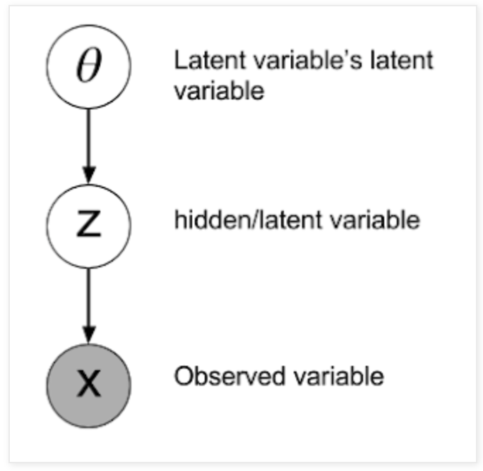
볼 수 있는 ("observable") variables (\( X \))와 숨겨진 ("hidden") variables (\( Z \))의 모음으로 아래의 그림과 같이 우리의 시스템을 만듭니다.

연결선 화살표는 Z에서 X로 향하게 되어 있습니다. 이는 두 variables이 conditional distribution \( \text{P(X|Z)} \)를 통해 서로 관련된다는 것을 의미합니다.
구체적인 예시를 통해 이해해 봅시다 : \( X \) 는 "raw pixel values of an image"라고 할 때, \(Z \)는 binary variable(\( Z=1 \), if X is an image of a cat)이라고 합시다.


Bayes' theorem 을 이용하면 random variables의 조합 간의 일반적인 관계를 얻을 수 있습니다.
$$ p(Z|X) = \frac{p(X|Z)p(Z)}{p(X)} $$
\( p(Z|X) \) - posterior probability : "이미지가 주어졌을때, 이것이 고양이일 확률이 얼마나 되는가?" 만약 우리가 \( z\) ~ \( P(Z|X) \)를 통해 \(z\) 값을 뽑아낼 수 있다면, 이것은 cat classifier로 사용될 수 있습니다.
\( p(X|Z) \) - likelihood : " \( Z\) 값이 주어 졌을 때, 이는 사진이 어떤 카테고리(고양이 or 고양이가아님)에 있을지 가능성을 계산합니다. 만약 우리가 \( x \) ~ \( P(X|Z) \)를 통해 \(x\) 값을 뽑아낼 수 있다면, 우리는 고양이 이미지를 만들어 내거나 고양이가 아닌 이미지를 만들어 낼 수 있습니다. 만약 이에 대해 더 알고 싶다면 다음의 글을 읽어보시길 바랍니다 [1], [2].
\(p(Z)\) - prior probability : Z에 대해 우리가 아는 정보를 뽑아냅니다. 예를들어, 우리가 가진 사진 데이터셋에서 고양이의 사진이 1/3이라면 \(p(Z=1)=\frac{1}{3}\) 이 되고 반대로, \(p(Z=0)=\frac{2}{3}\) 가 됩니다.
Hidden Variables as Priors
이 부분은 메인 주제와 크게 관련이 없기 때문에 메인 주제를 이어서 공부하시고 싶으시다면 아래로 스크롤하셔서 다음 부분(Problem Formulation)으로 넘어가 주시면 됩니다.
앞의 고양이 예시는 매우 일반적인 예시 입니다. 그러나 중요한 것은 hidden / observed variable 간의 구분이 다소 임의적이고 당신이 원하는 대로 모델을 변화시켜도 된다는 접입니다.(you're free to factor the graphical model however you like.)
그래서 우리는 Bayes' Theorem을 다음과 같이 swapping 해서 사용할 수 있습니다 :
$$ p(Z|X) = \frac{p(X|Z)p(Z)}{p(X)} $$
이제 "posterior"은 P(X|Z)가 되었습니다.
Hidden variables는 Bayesian_statistics framework를 통해 해석할 수 있습니다. 예를들어, 만약 \(X\)가 multivariate Gaussian이라고 믿는다면, hidden variable \(Z\)는 Gaussian distribution의 mean과 variance로 표현할 수 있습니다.
그리고 위의 식에서 The distribution over parameters \(P(Z)\)는 이제 \(P(X)\)에 대한 "prior distribution"로 사용됩니다.
\(X\)와 \(Z\)가 어떤 값을 표현하게 될지는 당신이 선택하는 것입니다. 예를 들어, \(Z\)는 "mean, cube root of variance, and \(X+Y\) where \( Y \sim \mathcal{N}(0,1)\)" 등이 될 수 있습니다. 좀 이상해 보일 수도 있지만 구조적으로 이것은 가능합니다.
심지어 당신의 시스템에 variables을 "add"할 수도 있습니다. The prior itself might be dependent on other random variables via P(Z|θ), which have prior distributions of their own P(θ), and those have priors still, and so on. Any hyper-parameter can be thought of as a prior. In Bayesian statistics, it's priors all the way down.
(이부분은 잘 이해가 되지 않습니다.)
Problem Formulation
Posterior inference 또는 hidden variable \(Z\)에 대한 계산이 가장 중요한 문제입니다.
몇 가지 posterior inference에 대한 예시 :
- Given this surveillance footage \(X\), did the suspect show up in it?
- Given this twitter feed \(X\), is the author depressed?
- Given historical stock prices \(X_{1:t-1}\), what will \(X_t\) be?
일반적으로 우리는 likelihood function \(P(X|Z)\) 그리고 priors \(p(Z)\)에 대한 함수들을 어떻게 계산하는지 알고 있다고 가정합니다.
그러나 여기서 문제는, 복잡한 과제에 대해서 \(P(Z|X)\)에서 값을 뽑아내는 방법을 모르거나 \(P(X|Z)\) 를 계산하지 못한다는 점입니다. \(P(X|Z)\)의 식을 안다고 할지라도, 이 식에 대한 연산이 매우 복잡하여 합리적인 시간 안에 계산하는 것이 불가능합니다.
그래서 수렴이 느리지만, sampling 기반의 MCMC 같은 접근 법을 시도해볼 수 있습니다.
Variational Lower Bound for Mean-field Approximation
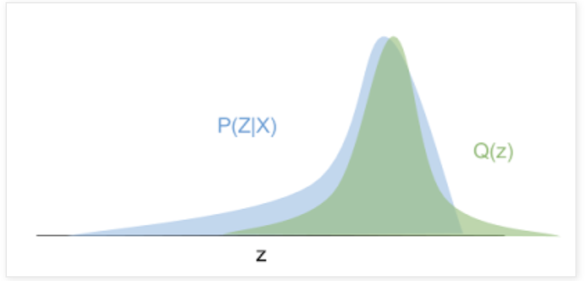
Variational inference의 배경이 되는 아이디어 : posterior inference 방법을 알고 있는 parametric distribution \(Q_{\phi}(Z|X)\)에 대한 inference를 실행한다고 생각해봅시다. 여기서 parameters \(\phi\)를 조절하여 \(Q_{\phi}\)가 \(P\)에 가능한 가까워지도록 합니다.
시각적으로 보면 아래의 그림 : 파란색 곡선이 true posterior distribution이라고 할 때, 녹색 distribution 은 variational approximation (Gaussian)이 됩니다. 우리는 이 녹색 distribution 을 최적화하여 파란색 density에 fitting 할 수 있습니다.
Distribution이 가깝다는 것은 어떤 의미일까요? Mean-field variational Bayes (가장 흔한 타입)은 Reverse KL Divergence를 두 distributions 사이의 distance metric으로 사용합니다.
$$ \textrm{KL}(Q_{\phi}(Z|X)||P(Z|X))=\sum_{z\in Z} q_{\phi}(z|x)log\frac{q_{\phi}(z|x)}{p(z|x)}$$
Reverse KL divergence는 \(P(Z)\)를 변형하여 \(Q_{\phi}(Z)\)로 만든데 필요한 정보의 양을 측정합니다. 우리는 이 정보의 양을 줄어드는 방향으로 \(\phi\) 값을 수정해갑니다.
Conditional distribution의 정의에 의해, \( p(z|x) = \frac{p(x,z)}{p(x)} \) 입니다. 그럼 이제 기존의 \(KL\) 표현식을 바꿔보자.
$$ \begin{align} KL(Q||P) & = \sum_{z\in Z}q_{\phi}(z|x)\textrm{log}\frac{q_{\phi}(z|x)p(x)}{p(z,x)}\\ & = \sum_{z\in Z}q_{\phi}(z|x)(\textrm{log}\frac{q_{\phi}(z|x)}{p(z,x)}+\textrm{log}p(x))\\ & = (\sum_{z}q_{\phi}(z|x)\textrm{log}\frac{q_{\phi}(z|x)}{p(z,x)})+(\sum_{z}\textrm{log}p(x)q_{\phi}(z|x))\\ & = (\sum_{z}q_{\phi}(z|x)\textrm{log}\frac{q_{\phi}(z|x)}{p(z,x)})+(\textrm{log}p(x)\sum_{z}q_{\phi}(z|x))\\ & = \textrm{log}p(x) + (\sum_{z}q_{\phi}(z|x)\textrm{log}\frac{q_{\phi}(z|x)}{p(z,x)})\\ \end{align} $$
$$\textrm{note} : \sum_z q(z) = 1$$
Variational parameters \(\phi\)에 대한 \(KL(Q||L)\) 를 최소화하기 위해, \(\textrm{log}p(x)\)는 \(\phi\)에 대해 고정된 값이기 때문에 놔둔 채로, 나머지 \(\sum_{z} q_{\phi}(z|x)\textrm {log}\frac {q_{\phi}(z|x)}{p(z, x)}\)을 최소화시켜야 합니다. 이제 이 정보 양을 distribution \(Q_{\phi}(Z|X)\)에 대한 expectation으로 재 작성해봅시다.
$$ \begin{align} \sum_{z}q_{\phi}(z|x)\textrm{log}\frac{q_{\phi}(z|x)}{p(z,x)} & = \mathbb{E}_{z\sim Q_{\phi}(Z|X)}[\textrm{log}\frac{q_{\phi}(z|x)}{p(z,x)}]\\ & = \mathbb{E}_{Q}[\textrm{log}q_{\phi}(z|x)-\textrm{log}p(z,x))] \\ & = \mathbb{E}_{Q}[\textrm{log}q_{\phi}(z|x)-(\textrm{log}p(z|x)+\textrm{log}(p(z)))]\quad (\textrm{via log} p(x,z) = p(x|z)p(z)) \\ & = \mathbb{E}_{Q}[\textrm{log}q_{\phi}(z|x)-\textrm{log}p(z|x)-\textrm{log}(p(z)))] \\ \end{align} $$
이것을 최소화 하는 것은 식에 마이너스를 붙여서 최대화 하는 것과 동일하다 :
$$ \begin{align}\textrm{maximize} \mathcal{L} & = - \sum_{z}q_{\phi}(z|x)\textrm{log}\frac{q_{\phi}(z|x)}{p(z,x)} \\ & = \mathbb{E}_{Q}[-\textrm{log}q_{\phi}(z|x)+\textrm{log}p(z|x)+\textrm{log}(p(z)))] \\ & = \mathbb{E}_{Q}[\textrm{log}p(z|x)+\textrm{log}\frac{p(z)}{q_{\phi}(z|x)}] \ \end{align}$$
문헌에서, \(\mathcal{L}\)은 variational lower baound 라고 알려져 있으며, 우리가 \(p(x|z),p(z),q(z|x)\)를 평가할 수 있다면 계산적으로 추적 가능하다. 만약 이를 조금더 직관적으로 바꾸면 :
$$ \begin{align} \mathcal{L} & = \mathbb{E}_{Q}[\textrm{log}p(z|x)+\textrm{log}\frac{p(z)}{q_{\phi}(z|x)}] \\ & = \mathbb{E}_{Q}[\textrm{log}p(z|x)]+\sum_Q q(z|x)\textrm{log}\frac{p(z)}{q_{\phi}(z|x)}] \quad \textrm{Definition of expectation}\\ & = \mathbb{E}_{Q}[\textrm{log}p(z|x)]-\textrm{KL}(Q(Z|X)||P(Z)) \quad \textrm{Definition of KL divedrgence}\\\end{align}$$
만약 샘플링 \(z \sim Q(Z|X)\)이 "encoding" 과정(observation \(x\) to latent code \(z\))이라면, 샘플링 \(x \sim Q(X|Z)\)은 "decoding" 과정(reconstructs the observation from \(z\))이 됩니다.
\(\mathcal{L}\)은 expected "decoding" likelihood와 \(\textrm{KL}\) divergence between the variational approximation and the prior on \(Z\)의 합이 됩니다. 만약 \(Q(Z|X)\)가 conditionally Gaussian이라고 가정하면, prior \(Z\)는 일반적으로 diagonal Gaussian distribution with mean 0 and standard deviation 1 으로 선택됩니다.
그렇다면 왜 \(\mathcal{L}\)을 variational lower bound라고 부를까요?
앞의 식을 그대로 가지고 와서 \(\mathcal{L}\)을 대입해 봅시다.
$$ \begin{align} \textrm{KL}(Q||P) & = \textrm{log}p(x) - \mathcal{L} \\ \textrm{log}p(x) & = \mathcal{L} + \textrm{KL}(Q||P)\\ \end{align}$$
이 수식의 의미는 다음과 같습니다. True distribution data point x의 log-likelihood 는 \(\mathcal{L}\)과 error term \(\textrm{KL}(Q||P)\)의 합이 됩니다. 여기서 이 error term은 \(X\)의 특정 값에서 \(Q(Z|X=x)\)와 \(P(Z|X=x)\)사이의 거리입니다.
\( \textrm{KL}(Q||P) \leq 0\) 이기 때문에 \(\textrm{log} p(x)\)는 무조건 \(\mathcal{L}\)보다 크게 됩니다. 그러므로 \(\mathcal{L}\)은 \(\textrm{log} p(x)\) lower bound 가 됩니다. \(\mathcal{L}\) 은 또한 아래의 식으로 표현되는 evidence lower bound(ELBO)라고도 불립니다.
$$\mathcal{L} = \textrm{log} p(x) - \textrm{KL}(Q(Z|X)||P(Z|X)) = \mathbb{E}_{Q}[\textrm{log}p(x|z)] - \textrm{KL}(Q(Z|X)||P(Z))$$
\(\mathcal{L}\)이 그자체로 \(\textrm{KL}\) divergence 항을 포함하고 있다는 것을 생각하면, 종합적으로 \(\textrm{log} p(x)\)에 두 개의 \(\textrm{KL}\) 항이 있습니다.
'Artificial Intelligence > Basic' 카테고리의 다른 글
| [ AI 기초 ] 1. Introduction for Artificial intelligence (0) | 2022.04.20 |
|---|---|
| Human Pose Estimation 이란? (2022) (0) | 2022.04.04 |
| 용어 정리 (인공지능, 머신러닝, 컴퓨터비전 분야) (0) | 2022.01.17 |
| 머신 러닝(Machine learning)이란 무엇인가? (supervised? or unsupervised?) (0) | 2020.03.21 |
| Chapter 1 - 2 다층 신경망 (MLP; Multi-Layer Perceptrons) (0) | 2020.03.08 |


